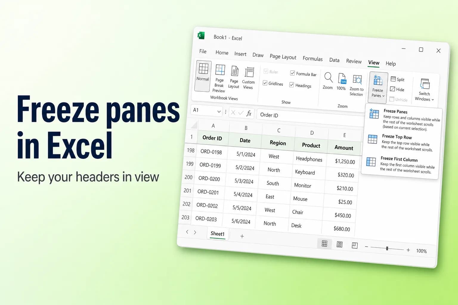
To freeze panes in Excel, go to View → Freeze Panes and pick Freeze Top Row, Freeze First Column, or Freeze Panes. The first two lock row 1 or column A. The third locks every row above and every column to the left of the cell you selected, so you can freeze several rows and columns at once.
The one thing that trips people up: Freeze Panes works from what is currently on screen. If you've scrolled down before freezing, the rows you scrolled past stay hidden and you can't scroll back to them. Press Ctrl+Home (Fn+Ctrl+Left Arrow on most Mac keyboards) to jump to the top of the sheet first.
| What you want to keep visible | Select this first | Then choose |
|---|---|---|
| Row 1 only | Any cell | Freeze Top Row |
| Column A only | Any cell | Freeze First Column |
| Row 1 and column A | Cell B2 | Freeze Panes |
| Rows 1 to 3 | Cell A4 (or all of row 4) | Freeze Panes |
| Columns A and B | Cell C1 (or all of column C) | Freeze Panes |
| Rows 1 to 2 and columns A to B | Cell C3 | Freeze Panes |
Freeze the top row or first column in Excel for Windows
This works the same way in Excel for Microsoft 365, Excel 2024, 2021, 2019 and 2016.
- Open the worksheet you want to work on. Freezing applies to one sheet at a time.
- Go to the View tab.
- In the Window group, click Freeze Panes.
- Choose Freeze Top Row to lock row 1, or Freeze First Column to lock column A.
A slightly darker line appears under row 1 (or to the right of column A). Scroll down or across and the frozen row or column stays put.
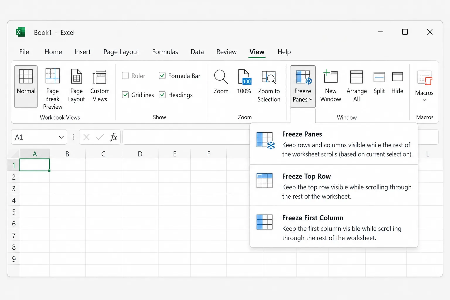
You can't combine Freeze Top Row and Freeze First Column: choosing one replaces the other. To lock both, use Freeze Panes with cell B2 selected, as shown in the next section.
Freeze multiple rows and columns at once
Freeze Panes freezes everything above and to the left of the selected cell. So the trick is to select the first cell that should still scroll.
- Scroll to the top of the sheet (
Ctrl+Home) so row 1 and column A are visible. - Click the cell just below the last row you want to freeze and just to the right of the last column you want to freeze. For example:
- C3 freezes rows 1 to 2 and columns A to B.
- A3 freezes rows 1 to 2 only (no columns).
- B1 freezes column A only (no rows).
- Go to View → Freeze Panes → Freeze Panes.
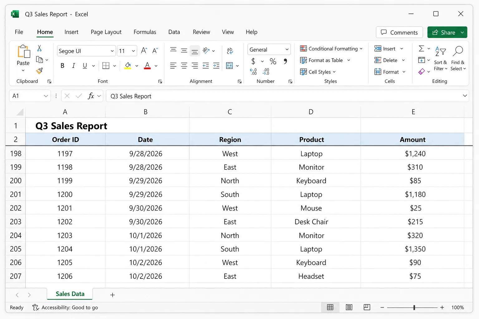
This is the setting you want when your sheet has a title in row 1 and the real column headings in row 2, or when an ID column and a name column both need to stay visible while you scroll across.
Keyboard shortcut
There's no single shortcut for Freeze Panes, but on Windows you can press the ribbon keys one after another (English versions of Excel):
Alt,W,F,Ffor Freeze Panes (or Unfreeze Panes when something is already frozen)Alt,W,F,Rfor Freeze Top RowAlt,W,F,Cfor Freeze First Column
Press the keys one at a time, not together.
How to unfreeze panes
Go to View → Freeze Panes → Unfreeze Panes. When panes are frozen, the first option in the menu changes from Freeze Panes to Unfreeze Panes. It removes all freezing from the current sheet.
To move the frozen line, unfreeze, select the new cell, and freeze again. Excel only allows one set of frozen panes per sheet.
Freeze panes in Excel for Mac
In Excel for Mac, the freeze commands are on the View tab. Depending on your version they appear as separate buttons or inside a Freeze Panes menu, but the names are the same:
- Go to the View tab.
- Click Freeze Top Row or Freeze First Column.
- To freeze several rows and columns, select the cell below and to the right of them (for example C3), then click Freeze Panes.
- To undo it, click Unfreeze Panes on the same tab.
If the buttons are greyed out, click Normal on the View tab. Freezing doesn't work in Page Layout view.
Freeze panes in Excel for the web
Excel for the web (excel.office.com or a file opened from OneDrive or SharePoint) uses the same menu as Windows:
- Go to View → Freeze Panes.
- Choose Freeze Top Row, Freeze First Column, or Freeze Panes (based on the selected cell).
- To remove it, choose View → Freeze Panes → Unfreeze Panes.
Frozen panes are saved with the workbook, so anyone who opens the file sees the same frozen rows, whether they use the web, Windows or Mac.
Freeze panes on iPhone, iPad or Android
The Excel mobile apps can freeze panes too, and the setting is saved in the file:
- iPad: select a cell, open the View tab, tap Freeze Panes, and choose the option you want.
- iPhone and Android phones: select a cell, tap the icon that opens the ribbon commands, switch from Home to View, and tap Freeze Panes.
The layout differs a little between devices and app versions, but the logic is the same.
Why Freeze Panes is greyed out or not working
You're still editing a cell. If you're typing in a cell or the formula bar, most of the ribbon is disabled. Press Enter or Esc and try again.
You're in Page Layout view. Freeze Panes isn't available in Page Layout view. Switch back with View → Normal, or click the Normal icon in the status bar at the bottom right.
The workbook is protected. If someone protected the workbook's window layout (an option under Review → Protect Workbook in older versions of Excel), you can't change frozen panes. Turn the protection off under Review → Protect Workbook, set up your frozen panes, then protect it again. The frozen panes stay in place after you re-protect.
You froze the wrong rows because the sheet was scrolled. Freeze Panes locks whatever is visible above the selected cell. If row 50 was at the top of the screen when you froze, rows 1 to 49 are now out of reach. Choose Unfreeze Panes, press Ctrl+Home, select the right cell, and freeze again.
The window is split. If you see grey split bars across the sheet, Split is on, and Freeze Panes will freeze at the split lines instead of at your selected cell. Click View → Split to turn it off, then freeze.
Your data is an Excel table. Tables have their own header trick: when you scroll down with a cell inside the table selected, Excel replaces the column letters (A, B, C) with the table's column names. That's why the headers can seem to "move" into the column bar. It isn't freezing, and it only works while your cursor is inside the table. If you want the header row locked at all times, use Freeze Panes as usual.
Freeze Panes vs Split
Both are on the View tab, but they do different jobs:
- Freeze Panes locks rows and columns in place so they never scroll.
- Split divides the window into two or four panes that each scroll on their own. It's useful for comparing row 10 with row 900 of the same sheet. Click Split again to remove it.
Repeating headers on every printed page is a different setting
Freezing panes only affects what you see on screen. To print your header row at the top of every page:
- Go to Page Layout → Print Titles.
- In Rows to repeat at top, select your header row (for example
$1:$1, or$1:$2for two rows). - For wide sheets, set Columns to repeat at left as well.
- Click OK, then check File → Print to preview it.
Frequently Asked Questions
How do I freeze the top two rows in Excel? Select cell A3 (or click the row number for row 3), then choose View → Freeze Panes → Freeze Panes. Rows 1 and 2 stay visible while you scroll.
How do I freeze both the top row and the first column? Select cell B2 and choose View → Freeze Panes → Freeze Panes. Picking Freeze Top Row and then Freeze First Column doesn't work, because the second replaces the first.
Can I freeze a row in the middle of the sheet? Not directly. Frozen panes always start at the top and left of what's on screen. If you scroll so that, say, row 20 is the top visible row and then freeze, rows above it are hidden until you unfreeze. For comparing two distant parts of a sheet, Split is usually the better tool.
Can I freeze the bottom row or a column on the right? No. Excel only freezes rows at the top and columns on the left. Use Split if you need to keep the bottom of a sheet in view.
Do frozen panes apply to every sheet in the workbook? No, each worksheet has its own setting. Freeze the panes on each sheet where you need them. The setting is saved with the file.
Is there a shortcut to freeze panes? On Windows, press Alt, W, F, F one after another to freeze panes at the selected cell, or Alt, W, F, R for the top row. Excel for Mac doesn't have a built-in shortcut, so use the View tab.
Make sense of a long sheet faster
Freezing the header row makes a long sheet readable, but you still have to scroll through hundreds of rows to spot what matters. CoreGPT for Excel can read the data for you: ask a question like "what stands out in Q3 sales?" and it points out the top regions, unusual drops and trends, right next to your workbook. It's free to start and works in Excel for the web, Windows and Mac.
 CoreGPT
Highlights:
- Europe leads at $184K, 23% over target
- 4 of 6 regions beat target
- North America is $7K short of target
Try it: CoreGPT for Excel
Related reading: