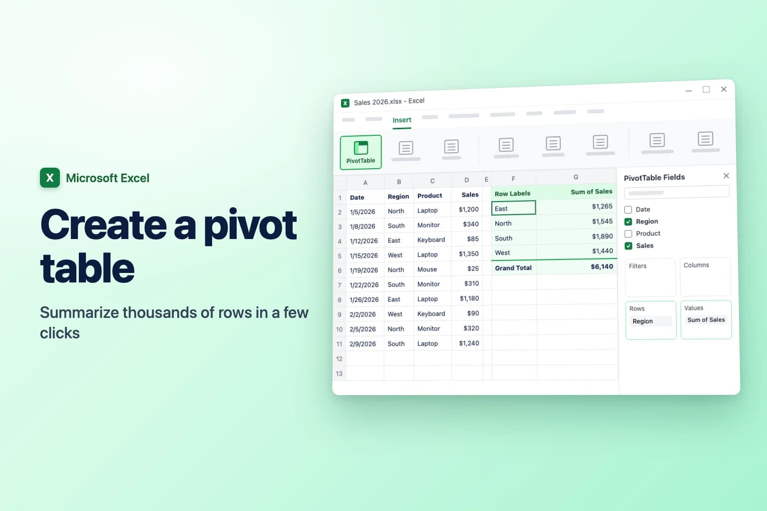
To create a pivot table in Excel, click any cell in your data and go to Insert → PivotTable → From Table/Range (in some versions you just click Insert → PivotTable). Check the range, choose New Worksheet, and click OK. Then, in the PivotTable Fields pane, tick a text field such as Region to put it in Rows and a number field such as Sales to put it in Values. Excel totals the sales for each region, no formulas needed.
What is a pivot table in Excel? It's a summary that groups and totals a list for you. You pick which column to group by (say, Region) and which to add up, count or average (say, Sales). You can rearrange it in seconds, and your original data never changes.
Most pivot table problems start before you click Insert: blank headings, empty rows or numbers stored as text. Two minutes of preparation prevents most of them.
| What you want | Where to do it |
|---|---|
| Create a pivot table | Insert → PivotTable → From Table/Range |
| Let Excel suggest one | Insert → Recommended PivotTables |
| Group by a field | Drag it to Rows (or Columns) |
| Add up, count or average a field | Drag it to Values, then Value Field Settings |
| Filter the whole report | Drag a field to Filters, or PivotTable Analyze → Insert Slicer |
| Group dates by month or year | Right-click a date → Group |
| Show new data | PivotTable Analyze → Refresh (Alt+F5) |
| Point it at a different range | PivotTable Analyze → Change Data Source |
Step 1: Prepare your data
The example in this guide is a sales list with the columns Date, Region, Product and Sales, one order per row. Before you start, check that:
- There's one header row. Every column has a short, unique heading. No blank headings, merged cells or second header row.
- There are no blank rows or columns inside the data. When Excel picks the range for you, it stops at the first completely empty row or column.
- Each column holds one type of data. Text like "n/a" or numbers stored as text in the Sales column make the pivot table count instead of sum.
- There are no subtotal or total rows. The pivot table makes its own.
Then format the list as a table: click a cell in it, press Ctrl+T (or Insert → Table), keep My table has headers ticked, and click OK. It's optional but worth it: rows you add to a table are included the next time you refresh the pivot table, while a plain range leaves them out.
Step 2: Insert the pivot table (Excel for Windows)
This works in Excel for Microsoft 365, Excel 2024, 2021, 2019 and 2016. The menu names below are from Microsoft 365; older versions open the same dialog when you click PivotTable.
- Click any cell inside your table or data range. Excel selects the whole list for you.
- Go to Insert → PivotTable → From Table/Range.
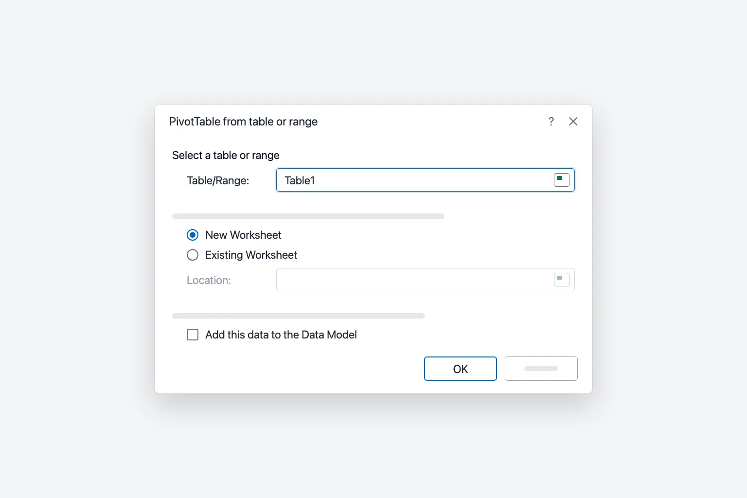
- In the PivotTable from table or range dialog (called Create PivotTable in older versions), check the Table/Range box. It shows the table name (for example
Table1) or a range such asSheet1!$A$1:$D$121. If the range looks wrong, select the correct cells on the sheet while the dialog is open. - Choose where the pivot table goes:
- New Worksheet puts it on a fresh sheet. This is the safest choice.
- Existing Worksheet puts it where you pick in the Location box. Leave enough empty space to the right and below, because the pivot table grows as you add fields.
- Leave Add this data to the Data Model unticked for now (it's for combining several tables).
- Click OK.
Excel opens a new sheet with an empty pivot table on the left and the PivotTable Fields pane on the right. If the pane disappears, click inside the pivot table or choose PivotTable Analyze → Field List.
Step 3: Build the report in the PivotTable Fields pane
The top of the pane lists every column heading of your data as a field. The bottom has four areas:
- Rows: the values you want down the left side (one row per region, product, month).
- Columns: the values you want across the top.
- Values: the numbers to calculate (sum, count, average).
- Filters: a field you want to filter the whole report by, shown above the pivot table.
To total sales by region:
- Tick Region. Text fields go to Rows automatically.
- Tick Sales. Number fields go to Values automatically and become Sum of Sales.
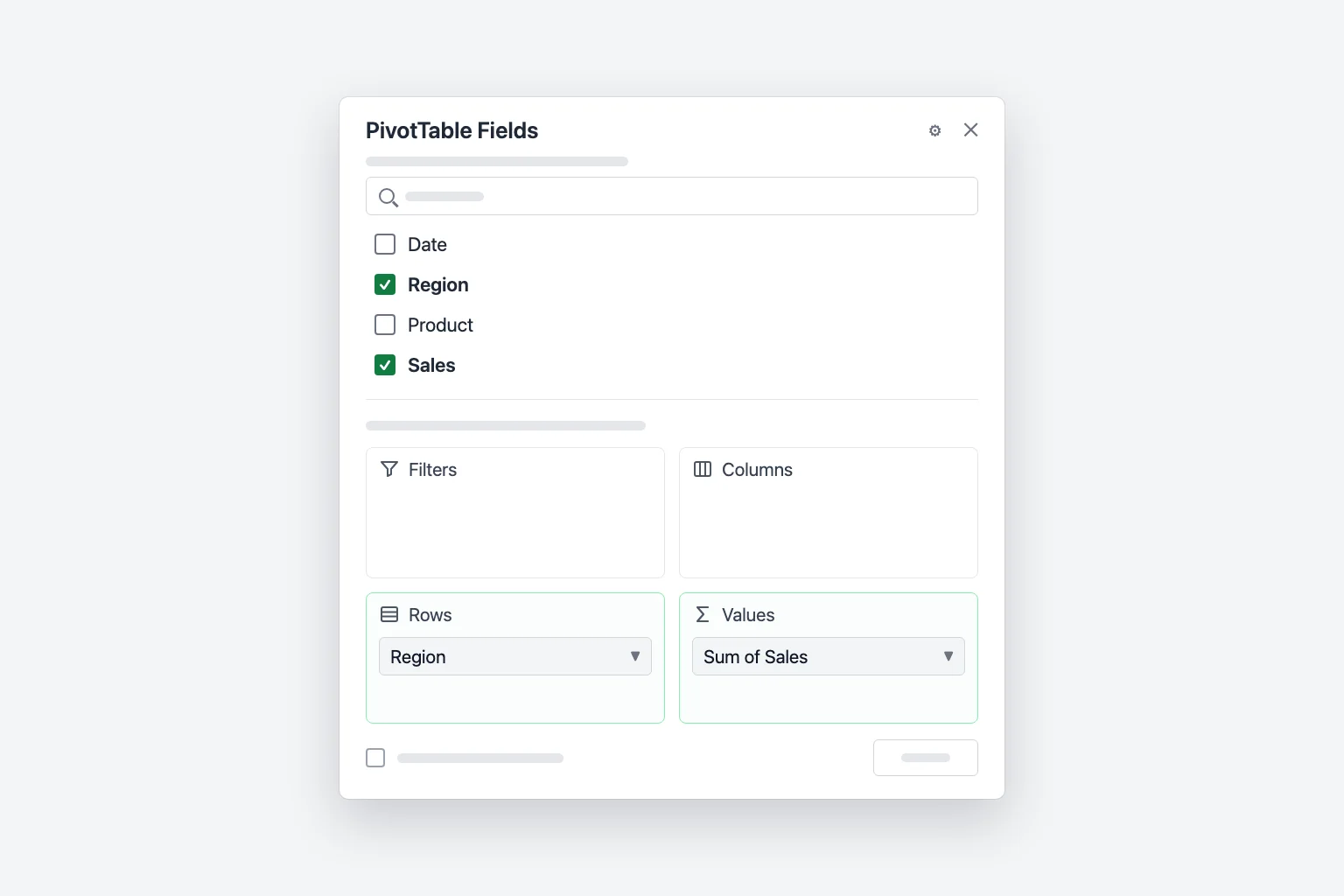
You now have one row per region and a Grand Total at the bottom. Excel lists the regions A to Z: in the example, East 1,265, North 1,545, South 1,890 and West 1,440, for a grand total of 6,140. The sums don't copy the currency format from your data at first; Step 4 shows how to add it.
Dragging gives you more control than ticking. Drag Product into Columns to see each product across the top, or into Filters to view one product at a time from a drop-down above the report. Put both Region and Product in Rows for a nested report. To remove a field, untick it or drag it out of its area.
Step 4: Change Sum to Count, Average or another calculation
Excel sums number fields and counts text fields. To change that:
- In the Values area, click Sum of Sales and choose Value Field Settings (or right-click any number in the pivot table and choose Value Field Settings).
- On the Summarize Values By tab, pick Count, Average, Max, Min or another option.
- Optionally type a clearer label in Custom Name, for example "Number of orders".
- Click Number Format to show the results as currency or with thousands separators.
- Click OK.
The Show Values As tab in the same dialog turns totals into shares, for example % of Grand Total. You can also drag a field into Values twice to show its sum and count side by side.
Step 5: Sort and filter the pivot table
- Sort by the totals: right-click any number in the Sum of Sales column and choose Sort → Sort Largest to Smallest. In the example, South moves to the top.
- Sort the labels: click the arrow next to Row Labels and choose Sort A to Z or Sort Z to A.
- Filter the rows: click the arrow next to Row Labels and untick the items you don't want, or use Value Filters → Top 10 to keep only the best performers.
- Slicers: click inside the pivot table, go to PivotTable Analyze → Insert Slicer, tick a field such as Product, and click OK. You get buttons that filter the report with one click. For dates, Insert Timeline adds a date slider.
Step 6: Group dates by month, quarter or year
When you add a date field to Rows, current versions of Excel for Windows often group it automatically into years, quarters and months. To choose the grouping yourself:
- Right-click any date in the pivot table and choose Group.
- In the Grouping dialog, select one or more options under By, for example Months and Years (select both if your data spans more than one year, otherwise January of every year lands in one row).
- Click OK.
To undo it, right-click a date and choose Ungroup. To stop automatic grouping, turn on Disable automatic grouping of Date/Time columns in PivotTables under File → Options → Data. If you see "Cannot group that selection", the date column contains blanks or text that only looks like a date: fix the source data and refresh.
Step 7: Refresh the pivot table and change its source
A pivot table doesn't update by itself when the data changes:
- Click inside the pivot table and choose PivotTable Analyze → Refresh, or right-click it and choose Refresh (
Alt+F5on Windows). - To refresh every pivot table in the workbook, choose PivotTable Analyze → Refresh → Refresh All (
Ctrl+Alt+F5).
If you added rows below a plain range, refreshing isn't enough. Go to PivotTable Analyze → Change Data Source → Change Data Source, select the new range (or type a table name such as Table1), and click OK. Pointing it at a table once avoids this for good.
Recommended PivotTables: let Excel build it for you
Not sure what to put where? Click inside your data and choose Insert → Recommended PivotTables. Excel previews ready-made summaries such as "Sum of Sales by Region" (in a dialog or a side pane, depending on your version). Pick one, then adjust it in the PivotTable Fields pane like any other pivot table.
Create a pivot table in Excel for Mac and Excel for the web
Excel for Mac: click a cell in your data and choose Insert → PivotTable. In the Create PivotTable dialog, check the range, choose New Worksheet or Existing Worksheet, and click OK. The PivotTable Fields pane has the same four areas. To change Sum to Count, open the field in Values and choose Field Settings. Refresh from the PivotTable Analyze tab or by right-clicking the pivot table.
Excel for the web: select your data and choose Insert → PivotTable. In the Insert PivotTable pane, choose New sheet or Existing sheet to build your own, or pick a suggestion (recommendations need a Microsoft 365 subscription). Tick fields in the PivotTable Fields pane as usual. To change the calculation, right-click a value and choose Summarize Values By. To update it, right-click the pivot table and choose Refresh.
Why your pivot table isn't working
"The PivotTable field name is not valid." At least one column in the source range has no heading, often an empty column at the edge of the range or a merged header cell. Give every column a heading, unmerge header cells, and make sure the range doesn't include a blank column.
New data doesn't show up. Refresh first. If the rows still aren't there, they're outside the source range: a fixed range like $A$1:$D$121 ignores row 122. Fix it with Change Data Source, ideally pointing to an Excel table.
Numbers are counted instead of summed. The value column contains blank cells or text, often numbers stored as text (they're left-aligned and may show a green triangle). Convert them to numbers (select them, click the warning icon, and choose Convert to Number), fill or remove the blanks, refresh, and switch the field back to Sum in Value Field Settings.
"Data source reference is not valid." The source range or table was deleted or renamed, or the workbook's file name contains square brackets. Fix the range with Change Data Source, or save the file under a name without [ ].
"A PivotTable report cannot overlap another PivotTable report." Two pivot tables on the same sheet grew into each other. Move one to another sheet (PivotTable Analyze → Move PivotTable) or leave more space between them.
Frequently Asked Questions
What is a pivot table used for? Summarizing long lists quickly: sales by region, orders per month, average cost per category. Instead of writing SUMIFS or COUNTIFS formulas, you drag fields into place.
How do I make a pivot table in Excel from multiple sheets? If the sheets have the same columns, the simplest way is to stack them into one table first. Otherwise, format each list as a table, insert a pivot table with Add this data to the Data Model ticked, choose All in the PivotTable Fields pane to see every table, and create relationships between them when Excel asks (they need a shared column, such as a product ID).
Does a pivot table update automatically? No. Refresh it with PivotTable Analyze → Refresh or Alt+F5, or turn on Refresh data when opening the file in PivotTable Options.
How do I delete a pivot table? Click inside it, choose PivotTable Analyze → Select → Entire PivotTable, and press Delete. If it's on its own sheet, you can also delete the sheet.
What's the difference between a pivot table and a table in Excel? An Excel table (Ctrl+T) is your data itself, with filters and automatic expansion. A pivot table is a read-only summary built from it, so to change a number you edit the source and refresh. They work best together.
Get answers from your data faster
A pivot table tells you the totals, but you still have to work out what they mean. CoreGPT for Excel reads your sheet for you: ask "what stands out in Q3 sales?" and it points out the strongest regions, unusual drops and trends, right next to your workbook. It's free to start and works in Excel for Windows, Mac and the web.
 CoreGPT
Highlights:
- Europe leads at $184K, 23% over target
- 4 of 6 regions beat target
- North America is $7K short of target
Try it: CoreGPT for Excel
Related reading: