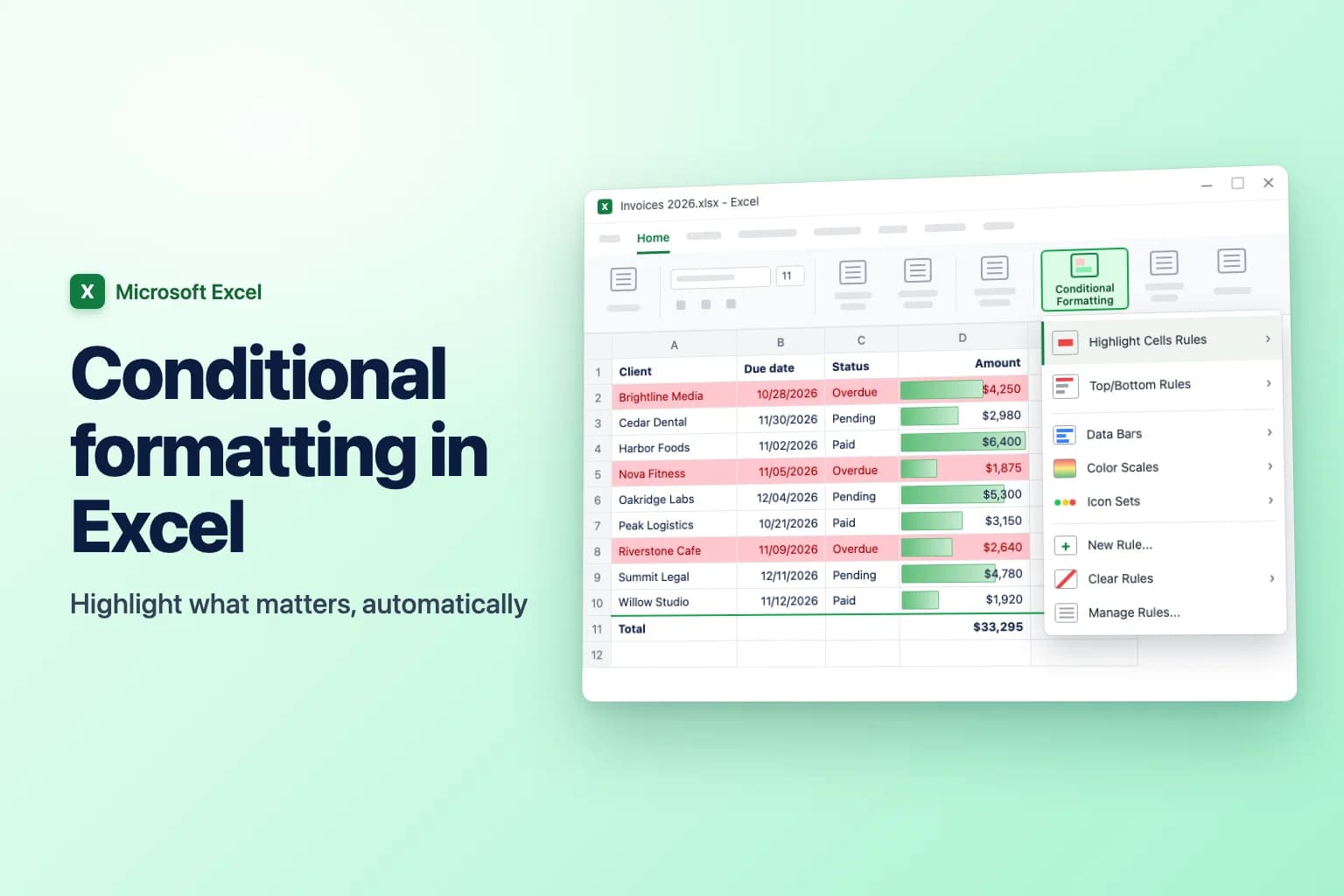
To use conditional formatting in Excel, select your cells, go to Home → Conditional Formatting, and pick a rule such as Highlight Cells Rules → Greater Than, Data Bars or Color Scales. For anything the menu doesn't cover, like highlighting a whole row or comparing two columns, choose New Rule → Use a formula to determine which cells to format and type a formula that returns TRUE for the cells you want formatted.
Most problems come from one detail: in a formula rule, the $ signs decide which cells the formula looks at. Get them right (usually $C2, with the column locked and the row free) and the rule works on every row. Get them wrong and Excel highlights the wrong cells, or none at all.
| What you want | Where to find it | Example |
|---|---|---|
| Highlight values above, below or between numbers | Highlight Cells Rules | Amounts greater than 5,000 |
| Highlight specific text or dates | Highlight Cells Rules → Text that Contains / A Date Occurring | "Overdue", or dates in the last 7 days |
| Find repeated entries | Highlight Cells Rules → Duplicate Values | Duplicate email addresses |
| Highlight the highest or lowest values | Top/Bottom Rules | Top 10 items, above average |
| Show size or trend at a glance | Data Bars, Color Scales, Icon Sets | Bars inside sales cells |
| Highlight a whole row or compare cells | New Rule → Use a formula… | =$C2="Overdue" |
Use the built-in conditional formatting rules
These steps are the same in Excel for Microsoft 365, 2024, 2021 and 2019 on Windows.
- Select the cells to format, for example the Amount column (D2:D10), without the header.
- Go to Home → Conditional Formatting. On Windows you can also press
Alt,H,Lone after another. - Point to Highlight Cells Rules and choose a rule:
- Greater Than, Less Than, Between or Equal To for numbers
- Text that Contains for words such as "Overdue"
- A Date Occurring for dates such as Yesterday, In the last 7 days, Next week or This month
- Duplicate Values to flag repeats (or switch the drop-down to Unique)
- Type the value, pick a format from the with list (such as Light Red Fill with Dark Red Text) or Custom Format.
- Click OK.

The rest of the menu works the same way:
- Top/Bottom Rules highlight the Top 10 Items, Top 10%, Bottom 10 Items, Bottom 10%, or values Above Average and Below Average. You can change the 10 to any number.
- Data Bars draw a bar inside each cell, longer for bigger values (Gradient Fill or Solid Fill).
- Color Scales shade cells from one color to another, for example red for low and green for high.
- Icon Sets add arrows, traffic lights or ratings based on where each value falls in the range.
To find or delete duplicates, see the guide to removing duplicates in Excel.
Highlight a whole row based on a cell value
Built-in rules only format the cells that meet the condition. To color the entire row when Status says "Overdue", you need a formula rule. Say your data is in A1:D100: Client in A, Due date in B, Status in C, Amount in D.
- Select the whole data range without the header row, starting from the top-left cell: click A2 and drag to D100.
- Go to Home → Conditional Formatting → New Rule.
- Under Select a Rule Type, choose Use a formula to determine which cells to format.
- In Format values where this formula is true, type:
=$C2="Overdue" - Click Format, open the Fill tab, pick a light red, and click OK.
- Check that the Preview shows your format, then click OK.
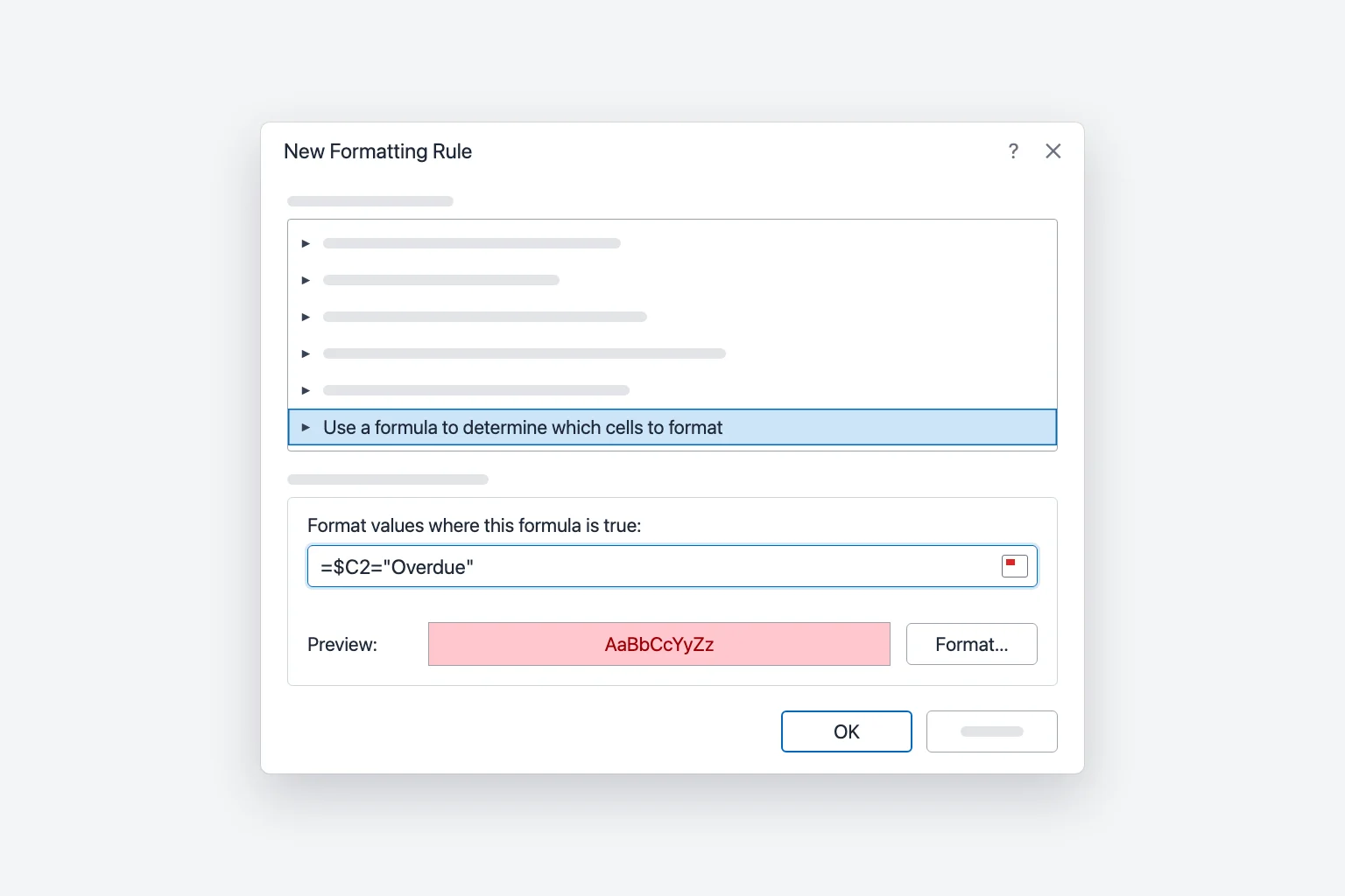
Every row where column C says "Overdue" now turns red from A to D, and the color follows when the status changes. The comparison isn't case-sensitive. If people type the status by hand, a drop-down list keeps the spelling consistent so the rule never misses a row.
Why the $ sign matters (the #1 mistake)
Excel writes your formula for the active cell, the first cell of your selection (A2 above), then adjusts it for every other cell, just like copying a formula down and across.
| Reference | As the rule moves across the range | Use it for |
|---|---|---|
$C2 | Column stays C, row changes | Whole-row rules (the usual choice) |
C2 | Column and row both change | Formatting a cell based on the cell next to it |
$C$2 | Never changes | A single threshold or input cell |
C$1 | Column changes, row stays 1 | Comparing each column with a value in row 1 |
With =C2="Overdue", cell A2 checks C2 but B2 checks D2, so only part of the row lights up. With =$C$2="Overdue", every cell checks C2, so the whole range is either all red or not at all.
Watch out: if you click a cell while typing the formula, Excel inserts an absolute reference like $C$2. Press F4 (on a Mac, Cmd+T or Fn+F4) to cycle through $C$2, C$2, $C2 and C2 until you get the one you need.
More formula examples
Use the same steps with these formulas. All assume your selection starts in row 2.
Format a cell based on another cell. In a sales sheet with Actual in column D and Target in column E, select D2:D100 and use:
=$D2<$E2
Every actual below its target turns red. Select A2:E100 instead to highlight the whole row.
Compare against one input cell. Put a threshold in H1, select D2:D100 and use =$D2>$H$1. $H$1 is fully absolute so every row looks at the same cell.
Highlight dates in the past. Select A2:D100 and use:
=$B2<TODAY()
Blank cells count as zero (a date in 1900), so empty due dates light up too. To skip blanks and paid invoices, use =AND($B2<>"",$B2<TODAY(),$C2<>"Paid").
Shade every other row. Select your data and use:
=MOD(ROW(),2)=0
This shades even rows (=1 for odd rows). Home → Format as Table with Banded Rows does the same without a rule.
Combine conditions. Use AND or OR, for example =AND($C2="Pending",$D2>5000) for large pending invoices. You don't need IF: the formula only has to return TRUE or FALSE.
Manage rules, rule order and Stop If True
Go to Home → Conditional Formatting → Manage Rules to open the Conditional Formatting Rules Manager.
- In Show formatting rules for, choose This Worksheet to see every rule on the sheet.
- Use Edit Rule or Delete Rule, or fix a rule's range in Applies to (for example
=$A$2:$D$100) and click Apply. - Use the Move Up and Move Down arrows to reorder rules. Rules higher in the list win.
If two rules set the same thing differently, such as two fill colors, the higher rule wins. If they don't clash (one makes the font bold, another fills the cell red), both apply. Rule formatting also overrides formatting you applied by hand.
Tick Stop If True to stop Excel from checking the rules below once that rule is true, which is handy for exceptions like "if Status is Paid, show nothing else". It isn't available for data bar, color scale or icon set rules.
To remove formatting, use Home → Conditional Formatting → Clear Rules → Clear Rules from Selected Cells or Clear Rules from Entire Sheet.
Copy conditional formatting to other cells
- Format Painter: select a formatted cell, click Home → Format Painter, then drag over the new cells. Double-click it to paint several ranges; press
Escto stop. - Paste Special: copy the cell, select the target, then Home → Paste → Paste Special → Formats.
- Extend the rule instead: edit the Applies to range in Manage Rules. This keeps one clean rule instead of several copies.
Excel for Mac and Excel for the web
Excel for Mac has the same Home → Conditional Formatting menu. For a formula rule, choose New Rule, change Style to Classic, pick Use a formula to determine which cells to format in the box below it, type the formula, and set Format with to Custom Format.
Excel for the web also uses Home → Conditional Formatting, but rules open in a Conditional Formatting pane instead of a dialog. For a formula rule, choose New Rule and set the rule type to Formula. Rules created on the desktop work in the browser and the other way around.
Why conditional formatting isn't working
It highlights the wrong rows (one row off). If your selection starts at A2, the formula must reference row 2. This usually happens when you include the header row or select from the bottom up.
Only one column is highlighted, or everything is. Check the dollar signs. Use $C2, not C2 or $C$2, for whole-row rules.
Numbers are stored as text. Imported values can look like numbers but be text (often with a small green triangle in the corner), so rules like Greater Than misbehave. Select the cells, click the warning icon and choose Convert to Number.
Text doesn't match. A trailing space ("Overdue ") or a different spelling won't equal "Overdue". Clean the data with TRIM, or use Text that Contains instead of Equal To.
Rules overlap or fight each other. Open Manage Rules, show This Worksheet, and check the order and Applies to ranges. Copying, pasting and inserting rows often splits one rule into many fragments.
The workbook got slow. Hundreds of fragmented rules, rules on entire columns (=$A:$D) and volatile functions like TODAY() or INDIRECT all add recalculation work. Delete duplicates and limit Applies to to the rows you use.
Frequently Asked Questions
How do I highlight a row based on a cell value in Excel? Select the data without headers, choose Home → Conditional Formatting → New Rule → Use a formula to determine which cells to format, enter =$C2="Overdue", and pick a fill. The $ before the column letter makes the whole row change color.
How do I apply conditional formatting based on another cell? Use a formula rule that points to that cell, for example =$D2<$E2 to highlight values below their target, or =$D2>$H$1 to compare every row with one input cell.
Can conditional formatting refer to another sheet? Yes, for example =$D2>Settings!$B$1. References to other workbooks aren't allowed.
Can I sort or filter by conditional formatting color? Yes. Turn on Data → Filter, open the column's filter arrow and choose Filter by Color or Sort by Color. It works with colors applied by rules.
How do I remove conditional formatting without deleting the data? Select the cells and choose Home → Conditional Formatting → Clear Rules → Clear Rules from Selected Cells. Your values stay as they are.
Let AI tell you what to highlight
Conditional formatting shows what you've already decided to look for. CoreGPT for Excel works the other way around: ask "what stands out in Q3 sales?" and it reads your data and points out top performers, unusual drops and trends, so you know which rules are worth setting up. It's free to start and runs inside Excel for Windows, Mac and the web.
 CoreGPT
Highlights:
- Europe leads at $184K, 23% over target
- 4 of 6 regions beat target
- North America is $7K short of target
Try it: CoreGPT for Excel
Related reading: