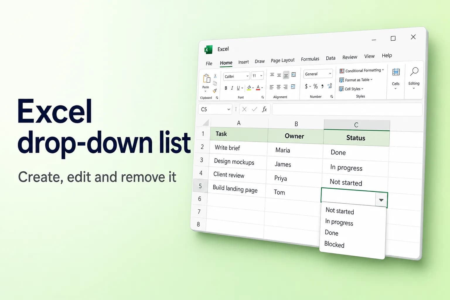
To create a drop-down list in Excel, select the cells, go to Data → Data Validation, set Allow to List, and in Source either type your items separated by commas or select the cells that contain them. Click OK, and each cell gets an arrow that opens your list.
The one choice that matters is where the items come from. A typed list is quick but awkward to change. If the list will grow, keep the items in an Excel table so every drop-down picks up new entries automatically.
| Source of the items | Example in the Source box | Updates automatically? | Best for |
|---|---|---|---|
| Typed list | Yes,No,Maybe | No, edit it by hand | Short lists that never change |
| Range of cells | =$F$2:$F$5 | Only if you edit within the range | Fixed lists kept on the sheet |
| Excel table | Select the table column's cells | Yes, as you add rows | Lists that grow over time |
| Spill range | =$H$2# | Yes, from a formula like UNIQUE | Lists pulled from existing data |
| Dependent list | =INDIRECT($A2) | Depends on the first choice | Category, then item |
Create a drop-down list step by step
These steps work in Excel for Microsoft 365, Excel 2021 and 2019 on Windows, and are nearly identical on Mac and in Excel for the web (differences below).
- Type your list items in a single column without blank cells, for example Not started, In progress, Done and Blocked in F2:F5. A separate sheet named "Lists" works well for this.
- Select the cell or cells where the drop-down should appear, for example C2:C50.
- Go to Data → Data Validation (in the Data Tools group). On Windows the keyboard shortcut is Alt, A, V, V.
- On the Settings tab, set Allow to List.
- Click in the Source box and select your items on the sheet (F2:F5, without the header). Excel fills in
=$F$2:$F$5. - Make sure In-cell dropdown is ticked. Leave Ignore blank ticked if empty cells are fine.
- Click OK.

Select one of those cells and an arrow appears beside it. Click it, or press Alt+Down Arrow (Option+Down Arrow on Mac), to open the list.

Typing the items instead of selecting cells
For a short, fixed list, type straight into Source: Yes,No,Maybe. Don't add spaces after the commas, or they become part of each item. If your regional settings use a comma as the decimal separator, Excel may expect semicolons instead (Yes;No;Maybe). The Source box holds up to 255 characters, so longer lists belong on the sheet.
Excel for Mac and Excel for the web
- Mac: Data → Data Validation (labeled Validate in the Tools group in some versions). The dialog has the same three tabs.
- Web: Data → Data Validation (under Data Tools on a narrow window), then the same Allow → List steps.
- Mobile: the iPhone, iPad and Android apps let you pick from drop-downs created on a computer.
Make the list grow automatically with a table
A plain range like $F$2:$F$5 won't include an item you type in F6. Turn the list into a table and it will:
- Click a cell in your list and press
Ctrl+T(Cmd+Ton Mac). Tick My table has headers and click OK. - Create the drop-down as above, selecting the table's data cells (without the header) in Source.
- Type a new item in the row directly below the table. The table expands, and every drop-down based on it shows the new item.
You can't type a table reference such as =Table1[Status] directly into Source; Excel rejects it. Select the cells instead, or use =INDIRECT("Table1[Status]").
A named range also works: select the items, type a name such as Statuses in the Name Box (left of the formula bar), press Enter, and use =Statuses as the source.
Build a dynamic list from existing data with UNIQUE
If the options should come from data you already have, for example every customer name in column A, let a formula build the list. In Excel for Microsoft 365, Excel 2021 or later, or Excel for the web:
- In an empty cell, say H2, enter
=SORT(UNIQUE(FILTER(A2:A500,A2:A500<>""))). The sorted, duplicate-free list spills down from H2 (theFILTERpart leaves out empty cells, which would otherwise show up as a 0). - Create the drop-down with Source set to
=$H$2#.
The # tells Excel to use the whole spill range, however long it gets, so new names appear in the drop-down automatically. You can't put UNIQUE itself in the Source box, which is why the helper cell is needed. For more on UNIQUE, see How to Remove Duplicates in Excel.
Use a list on another sheet
While the Source box is active, click the other sheet's tab and select the cells; Excel writes something like =Lists!$A$2:$A$10. You can then hide the Lists sheet (right-click its tab → Hide) so nobody edits it by accident. A source in a different workbook only works while that workbook is open, so keep the list in the same file.
Create a dependent (cascading) drop-down with INDIRECT
A dependent drop-down changes its options based on another cell: pick Fruit in column A, and column B offers only fruits.
- On your Lists sheet, put each category in a header with its items below. For example, Fruit in D1 with Apple, Banana, Cherry below it, and Vegetables in E1 with Carrot, Leek, Pea.
- Select D1:E4 and go to Formulas → Create from Selection. Tick only Top row and click OK. Excel creates a named range for each column, named after its header.
- In A2 on your main sheet, create a normal drop-down whose source is the two header cells,
=Lists!$D$1:$E$1(the category names). - Select B2, open Data → Data Validation, choose List, and enter
=INDIRECT($A2)as the source. - If Excel warns that the source currently evaluates to an error, click Yes. That's only because A2 is still empty.
Names can't contain spaces, so Create from Selection turns "Dairy products" into Dairy_products. For categories with spaces, use =INDIRECT(SUBSTITUTE($A2," ","_")) instead.
Add an input message and an error alert
- Input Message: tick Show input message when cell is selected and enter a title and short message, such as "Choose the task status". It appears whenever someone selects the cell.
- Error Alert: tick Show error alert after invalid data is entered and choose a Style. Stop blocks anything not in the list, while Warning and Information show your message but let the entry through.
Note that validation only checks what people type. Pasting over a cell replaces its drop-down along with its contents.
Search a drop-down by typing
In current Microsoft 365 versions of Excel, typing in a drop-down cell filters the list to items that contain those letters, which makes long lists much faster. Excel 2021 and earlier don't have this.
Edit, copy or remove a drop-down list
Add or change items. For a table, type the new item below it. For a range, edit the cells, then reopen Data → Data Validation and adjust Source if the range got longer. For a typed list, edit the text in Source. Tick Apply these changes to all other cells with the same settings to update every matching drop-down at once.
Copy the drop-down to more cells. Drag the fill handle down, or copy the cell, select the destination, and choose Home → Paste → Paste Special → Validation to copy only the drop-down without the value.
Remove a drop-down. Select the cells, go to Data → Data Validation, click Clear All, then OK. Any values already in the cells stay. To find every cell that has a drop-down, use Home → Find & Select → Data Validation.
Why your drop-down isn't working
- No arrow appears. Open Data → Data Validation and tick In-cell dropdown. The arrow also only shows when the cell is selected. If arrows are missing everywhere, check File → Options → Advanced → Display options for this workbook and set For objects, show to All.
- New items don't show up. The source is a fixed range. Extend it, or convert the list to a table or a spill range so it grows by itself.
- Data Validation is greyed out. The sheet is protected (Review → Unprotect Sheet), the workbook uses the legacy shared workbook feature, several sheets are grouped (click a single sheet tab), or you're still editing a cell (press Enter or Esc).
- The list shows blanks. The source range includes empty cells. Shrink it or use a table.
- Someone typed a value that isn't in the list. The Error Alert style is Warning or Information, or the alert is turned off. Switch it to Stop.
Frequently Asked Questions
How do I add a drop-down list to a whole column? Select the column range you need, such as C2:C1000, before opening Data Validation. If your data is in a table, a drop-down applied to the column carries over to new rows automatically.
Can an Excel drop-down list allow multiple selections? Not with built-in Data Validation. Each cell holds one choice. Picking several values requires a VBA macro or a different layout, such as one column per option.
How many items can a drop-down list have? A list from cells can hold thousands of items, though long lists are hard to scroll. A typed list is limited by the 255-character Source box.
How do I make a drop-down with Yes and No? Set Allow to List and type Yes,No in Source.
How do I remove a drop-down but keep the values? Select the cells, go to Data → Data Validation → Clear All, and click OK. The current values remain as plain text.
Keep your list data clean
A drop-down only works well when the data behind it is consistent. CoreGPT for Excel lets you describe a cleanup in plain English, such as "remove duplicate customers and fix the different spellings of each country", and does it inside your workbook, so the lists you build drop-downs from stay tidy. It's free to start and works in Excel for the web, Windows and Mac.
 CoreGPT
Done. I made these changes:
- Removed 12 duplicate rows
- Changed “US”, “DE”… to full names
- Formatted phone numbers
Try it: CoreGPT for Excel
Related reading: