In the XLOOKUP vs VLOOKUP choice, use XLOOKUP if everyone who opens the file has Excel for Microsoft 365, Excel 2021 or later, or Excel for the web. It does everything VLOOKUP does with fewer mistakes: exact match by default, it can look left, and it doesn't break when you insert a column. Use VLOOKUP only when the workbook has to work in Excel 2019 or older.
That compatibility point is the main caveat. XLOOKUP doesn't exist in Excel 2016 or 2019, so a file full of XLOOKUP formulas shows #NAME? errors for anyone still on those versions.
| VLOOKUP | XLOOKUP | |
|---|---|---|
| Look left (return a column left of the lookup column) | No | Yes |
| Default match type | Approximate (unless you add FALSE) | Exact |
| Survives inserting or deleting columns | No, the column number stays fixed | Yes, ranges adjust |
| Custom "not found" message | Needs IFNA or IFERROR | Built in (if_not_found) |
| Return several columns at once | Not easily | Yes, results spill |
| Search from the last match up | No | Yes (search_mode -1) |
| Approximate match | Data must be sorted ascending | Next smaller or larger, no sorting needed |
Wildcards (*, ?) | Yes, with exact match | Yes, with match_mode 2 |
| Horizontal lookups | No, that's HLOOKUP | Yes, same function |
| Speed | No practical difference in typical workbooks | Same, plus optional binary search on sorted data |
| Available in | Every version of Excel | Microsoft 365, Excel 2021, Excel 2024, Excel for the web, mobile apps |
The syntax side by side
=VLOOKUP(lookup_value, table_array, col_index_num, [range_lookup])
=XLOOKUP(lookup_value, lookup_array, return_array, [if_not_found], [match_mode], [search_mode])
The big difference is how you tell Excel where the answer is. VLOOKUP takes a whole table and a column number counted from the left edge of that table. XLOOKUP takes two separate ranges: the column to search in and the column to return from.
The same lookup written both ways
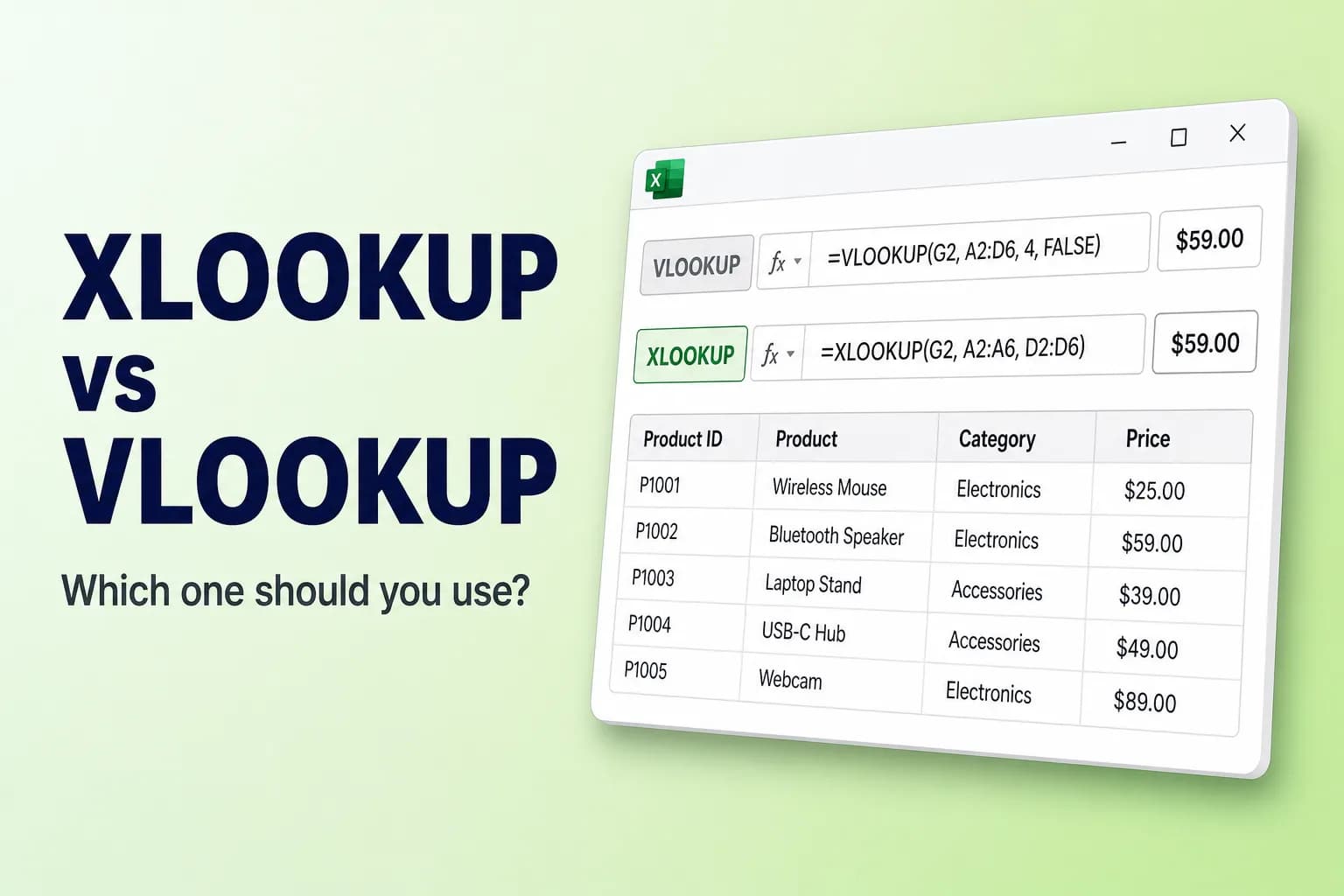
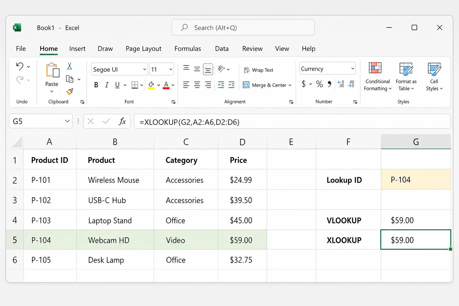
Here's a small product list in A1:D6, with a product ID typed in G2:
| A | B | C | D | |
|---|---|---|---|---|
| 1 | Product ID | Product | Category | Price |
| 2 | P-101 | Wireless Mouse | Accessories | $24.99 |
| 3 | P-102 | USB-C Hub | Accessories | $39.50 |
| 4 | P-103 | Laptop Stand | Office | $45.00 |
| 5 | P-104 | Webcam HD | Video | $59.00 |
| 6 | P-105 | Desk Lamp | Office | $32.75 |
To find the price of P-104:
=VLOOKUP(G2, A2:D6, 4, FALSE)
=XLOOKUP(G2, A2:A6, D2:D6)
Both return $59.00. VLOOKUP searches the first column of A2:D6 and returns the 4th column; FALSE forces an exact match. XLOOKUP searches A2:A6 and returns the matching cell from D2:D6, with exact match as the default.
If you'll copy the formula down a column, lock the table with absolute references, for example =XLOOKUP(G2, $A$2:$A$6, $D$2:$D$6). Press F4 on Windows or Cmd+T on Mac while the cursor is in a reference to add the $ signs.
VLOOKUP's two classic pitfalls
1. Forgetting FALSE (or 0)
The last VLOOKUP argument is optional, and when you leave it out Excel uses approximate match. With approximate match, VLOOKUP assumes the first column is sorted and returns the closest value that's less than or equal to what you searched for, without any warning.
Try =VLOOKUP("P-110", A2:D6, 4) on the table above. P-110 doesn't exist, but instead of #N/A you get $32.75, the price of P-105, because "P-105" is the closest smaller value. On unsorted data the results can be even more random.
Always end an exact-match VLOOKUP with FALSE or 0. XLOOKUP avoids the problem because it uses exact match unless you ask otherwise.
2. The hard-coded column number
The 4 in the VLOOKUP formula is just a number. If someone inserts a Supplier column between Product and Category, the table becomes A:E, Price moves to column E, and the formula still returns the 4th column, which is now Category. You'd see "Video" instead of $59.00.
XLOOKUP points at the price column itself (D2:D6), so Excel updates it to E2:E6 automatically and the answer stays correct.
What XLOOKUP can do that VLOOKUP can't
Look left
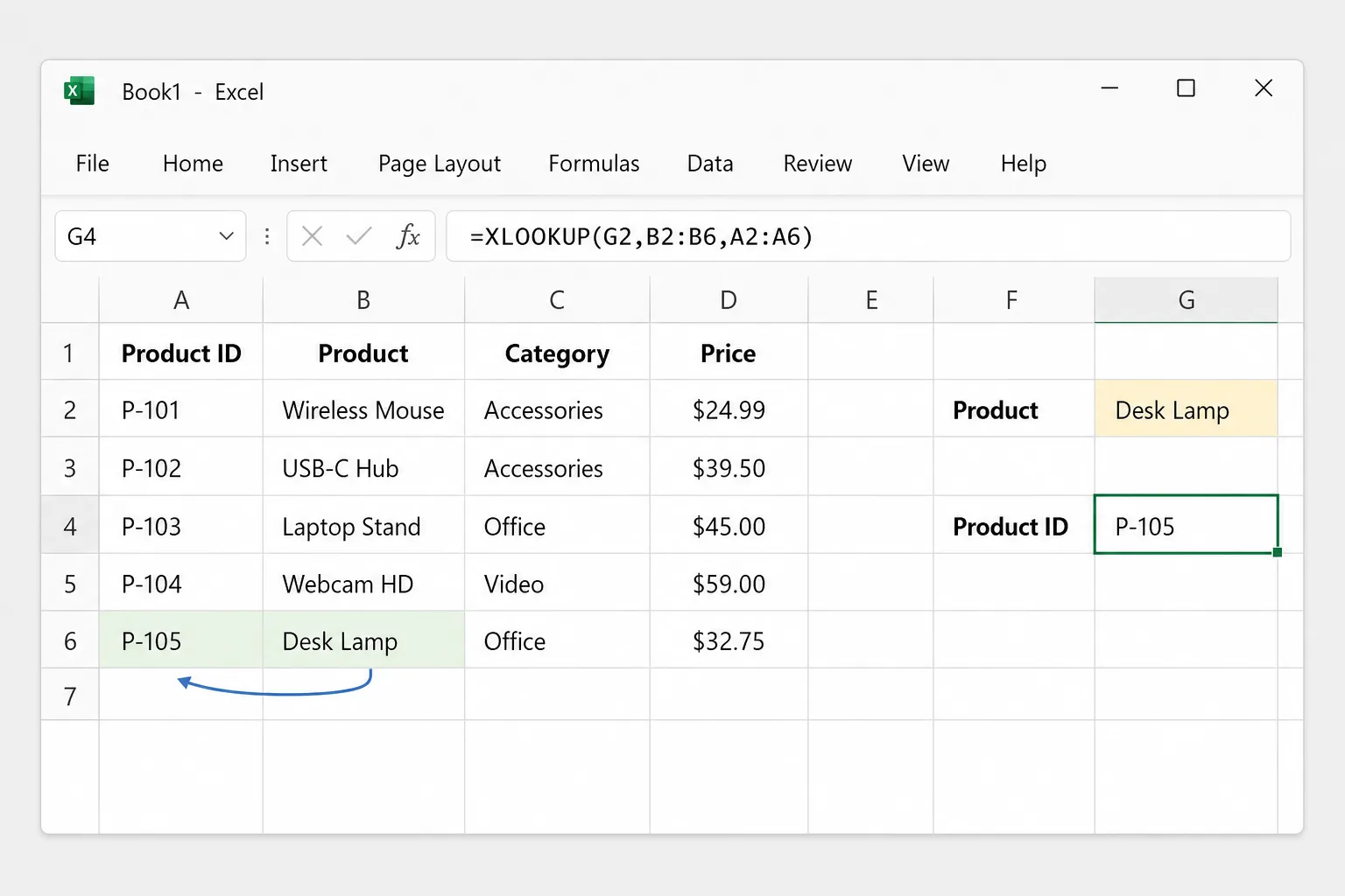
VLOOKUP can only return columns to the right of the lookup column. XLOOKUP doesn't care about direction. To find the product ID for a product name in G2:
=XLOOKUP(G2, B2:B6, A2:A6)
With "Desk Lamp" in G2, this returns P-105, even though column A is to the left of column B.
Show a friendly message when nothing is found
=XLOOKUP(G2, A2:A6, D2:D6, "Not found")
The VLOOKUP equivalent needs a wrapper: =IFNA(VLOOKUP(G2, A2:D6, 4, FALSE), "Not found").
Return several columns in one formula
=XLOOKUP(G2, A2:A6, B2:D6)
For P-104 this spills Webcam HD, Video and $59.00 into three cells side by side. Leave those cells empty, or you'll get a #SPILL! error.
Find the last match instead of the first
In a log where the same customer appears many times, set search_mode to -1 to search from the bottom up and get the most recent entry:
=XLOOKUP(G2, A2:A500, C2:C500, "Not found", 0, -1)
Approximate match without sorting
For tiered prices or commission rates, VLOOKUP's approximate match only works if the first column is sorted ascending. XLOOKUP's match_mode -1 (exact match, or the next smaller item) and 1 (exact match, or the next larger item) don't need sorted data. With minimum order amounts in J2:J5 and discounts in K2:K5:
=VLOOKUP(B2, J2:K5, 2, TRUE)
=XLOOKUP(B2, J2:J5, K2:K5, , -1)
Wildcards
Both support * and ?, but XLOOKUP needs match_mode 2 to treat them as wildcards:
=VLOOKUP("Desk*", B2:D6, 3, FALSE)
=XLOOKUP("Desk*", B2:B6, D2:D6, , 2)
Both return $32.75 for Desk Lamp.
INDEX/MATCH: the classic alternative
Before XLOOKUP, the standard fix for VLOOKUP's limits was INDEX with MATCH. It looks left, survives inserted columns, and works in every version of Excel, which makes it the best choice for files that must open in Excel 2019 or older:
=INDEX(D2:D6, MATCH(G2, A2:A6, 0))
=INDEX(A2:A6, MATCH(G2, B2:B6, 0))
The first returns the price for the ID in G2; the second is the look-left example. The 0 in MATCH means exact match, and like VLOOKUP's FALSE, it's easy to forget. XLOOKUP is simply the shorter, safer version of the same idea.
How to convert VLOOKUP formulas to XLOOKUP
There's no built-in converter, but the translation is mechanical:
- Find your VLOOKUPs: press
Ctrl+F(Cmd+Fon Mac), type VLOOKUP, click Options if the extra settings are hidden, set Look in to Formulas, and click Find All. - Keep the first argument (the lookup value) as it is.
- Replace the table with its first column as
lookup_array. - Replace the column number with the matching column as
return_array. Column 5 of a table that starts in column A is column E. - Drop
FALSE. If the original ended inTRUEor had no last argument, addmatch_mode-1 to keep the "next smaller" behavior.
For example:
=VLOOKUP(A2, Products!$A$2:$F$500, 5, FALSE)
=XLOOKUP(A2, Products!$A$2:$A$500, Products!$E$2:$E$500)
Test a few results against the old formula before converting a whole sheet. Approximate-match VLOOKUPs on unsorted data may have been returning wrong values all along, so XLOOKUP's answers can legitimately differ.
What happens when an XLOOKUP file opens in Excel 2016 or 2019
The workbook opens, but those versions don't know the function. In the formula bar it appears as =_xlfn.XLOOKUP(...). The cells may still show the last saved results at first, but as soon as the formula recalculates, it returns #NAME?.
If you share files with people on older versions:
- Use INDEX/MATCH or VLOOKUP instead, or
- Send a copy with the results pasted as values (Copy → Paste Special → Values).
The same applies to other newer functions like FILTER, UNIQUE and XMATCH.
XLOOKUP in Google Sheets
Google Sheets has XLOOKUP too, with the same argument order: =XLOOKUP(search_key, lookup_range, result_range, [missing_value], [match_mode], [search_mode]). The formulas in this post work there as written, so XLOOKUP is a safe choice for files that move between Excel and Sheets.
Why your lookup returns #N/A or the wrong value
- Extra spaces. "P-104 " with a trailing space doesn't match "P-104". Clean the data with
TRIM. - Numbers stored as text. An ID typed as text won't match the same ID stored as a number. Look for the green triangle in the corner of the cell and convert the column to one type.
- Missing FALSE in VLOOKUP. You get a plausible but wrong answer instead of
#N/A. - Ranges that moved when you copied the formula. Use
$absolute references for the lookup table. #REF!from VLOOKUP. The column number is larger than the number of columns in the table.#VALUE!from XLOOKUP. The lookup and return ranges are different sizes, for example A2:A6 and D2:D60.#NAME?The function name is misspelled, or the file is open in a version without XLOOKUP.
Frequently Asked Questions
Is XLOOKUP better than VLOOKUP? Yes, for almost every use. It's exact match by default, looks in any direction, doesn't break when columns move, and handles missing values without a wrapper. VLOOKUP's only real advantage is that it works in every version of Excel.
Is XLOOKUP faster than VLOOKUP? In everyday workbooks you won't notice a difference. On very large sorted lists, XLOOKUP's binary search modes (search_mode 2 or -2) can speed things up, but they return wrong results if the data isn't sorted.
Why does XLOOKUP show #NAME? on my computer? Your Excel version doesn't include XLOOKUP. It's in Microsoft 365, Excel 2021 and later, and Excel for the web, but not in Excel 2019 or 2016. Use INDEX/MATCH instead.
Does XLOOKUP replace HLOOKUP too? Yes. If the lookup and return ranges are rows instead of columns, XLOOKUP searches horizontally with the same syntax.
Can XLOOKUP return all matches, not just the first? No, it returns one match (or one row of columns). To get every matching row, use FILTER, for example =FILTER(A2:D6, C2:C6="Office").
Should I still learn VLOOKUP? It's worth recognizing, because you'll find it in older workbooks and templates. For new formulas, learn XLOOKUP, and keep INDEX/MATCH in mind for files that must open in older Excel.
Let AI write the lookup for you
Lookup formulas are where small details, like a missing FALSE or a shifted range, cause the most quiet errors. CoreGPT for Excel lets you describe what you need, such as "find the price for the product ID in G2" or "flag each row as above or below target", and writes the formula into your sheet with a short explanation. It's free to start and works in Excel for Windows, Mac and the web.
 CoreGPT
Use this formula and fill it down:
=IF(C2>=D2,"Above","Below")Try it: CoreGPT for Excel
Related reading: